At its heart, the most fundamental timesheet excel formula is =(EndTime - StartTime) * 24. This little powerhouse calculates the total hours worked by converting Excel's native time value into a simple decimal number. But hold on. Before you start plugging that into your cells, we need to talk about the foundation.
A powerful formula is useless on a shaky foundation, and a poorly structured timesheet is a disaster waiting to happen. Getting the setup right from the start will save you countless headaches trying to fix broken calculations later.
Building A Reliable Timesheet From The Ground Up
Let's start with the basics. Every solid timesheet needs a few non-negotiable columns. Think of these as the skeleton of your entire system.
You'll want clear, dedicated headers for at least these items:
- Date: The specific day the work was done.
- Start Time: When the clock-in happened.
- End Time: The time of clock-out.
- Break Duration: Total time for any unpaid breaks.
- Total Hours Worked: This is where our first formula will live.
Set Up Essential Cell Formatting
One of the most common trip-ups I see is incorrect cell formatting. If you just subtract one time from another, Excel might spit out something weird like "0.33" instead of a clean "8:00." That's because Excel thinks of time as a fraction of a 24-hour day. You have to explicitly tell it how to display your data.
This infographic lays out the whole workflow perfectly. It’s all about getting the structure and formatting locked in before you even think about the math.
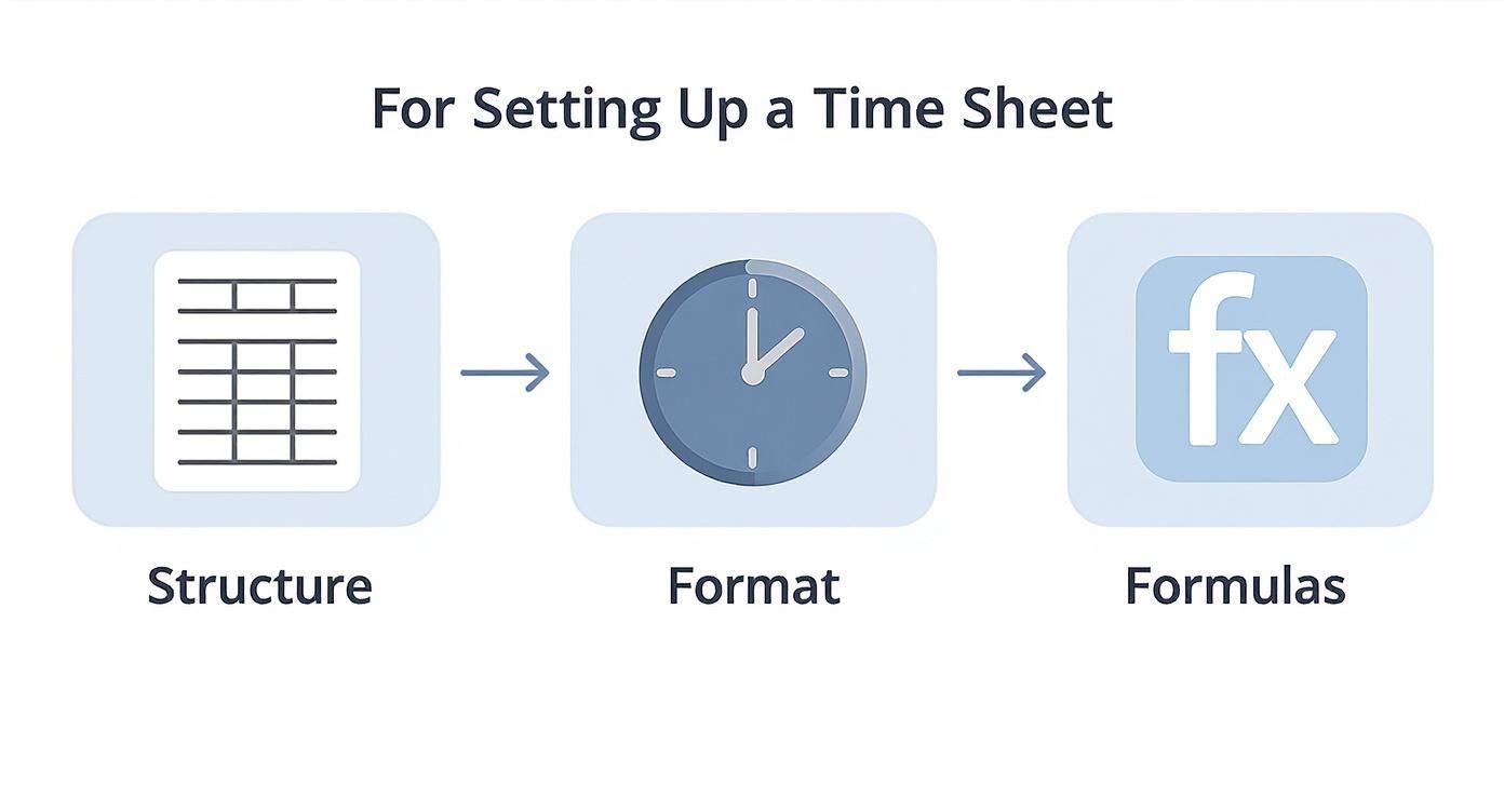
As you can see, the process flows from a solid setup to accurate calculations—not the other way around. To make this happen, you'll need to get comfortable with Excel's custom formatting options.
To avoid the most common formatting errors that throw off payroll calculations, you need to apply the right custom formats to your cells. Here’s a quick-reference table with the essentials.
Essential Time and Number Formats for Timesheets
| Data Type | Excel Format | Example | Purpose |
|---|---|---|---|
| Time (In/Out) | h:mm AM/PM | 9:00 AM | Displays time in a standard, readable 12-hour format. |
| Time Duration (Hours) | [h]:mm | 8:30 | Correctly shows total hours, even if they exceed 24. |
| Decimal Hours | Number or General | 8.50 | Converts time into a decimal for easy payroll calculation. |
| Currency | Currency or $ | $150.00 | Formats pay rates and total pay with the correct currency symbol. |
Getting these formats right is the single most important step for an accurate timesheet. It ensures that when you calculate pay, you're working with the right numbers.
Advanced Setup For Easier Formulas
Once the basics are nailed down, you can add a few extra touches that will make your formulas much cleaner and easier to read. For example, instead of hardcoding numbers into your formulas, use Named Ranges.
Creating a named range for something like PayRate or OvertimeThreshold is a game-changer. Instead of a clunky formula like =IF(E2>40, ...), you get to write something intuitive and self-explanatory like =IF(TotalHours>OvertimeThreshold, ...). It’s a small change that makes your spreadsheet infinitely more manageable.
This kind of structural thinking isn't just for timesheets; it's a core skill for mastering spreadsheet management in general. It's the same logic you'd apply when creating an efficient employee directory using Excel.
Maintaining this discipline is what separates a functional timesheet from a frustrating one. You can learn more about the https://www.timetackle.com/why-you-need-to-maintain-a-timesheet-pros-and-cons-of-timesheet-in-excel-or-google-docs/.
Formulas to Calculate Daily and Weekly Hours
Once your timesheet is structured and properly formatted, it's time to make it work for you. This is where we plug in the formulas that do all the heavy lifting, turning those raw start and end times into clean data ready for payroll.
The first and most basic task is figuring out how long a single shift was. Let's say an employee starts at 9:00 AM (cell B2) and clocks out at 5:00 PM (cell C2). The obvious formula is a simple subtraction: =C2-B2. This will give you a result like "8:00," which looks right, but it's still in Excel's native time format. That's not very helpful when you need to calculate pay.

The Magic of Multiplying by 24
To get that "8:00" into a decimal number like 8.0, you need to multiply the result by 24. Why? Because Excel stores time as a fraction of a 24-hour day. So, 12:00 PM is 0.5, 6:00 AM is 0.25, and so on. Multiplying by 24 converts that fraction back into the hours we actually use.
So, the go-to formula for calculating total daily hours becomes:
=(C2-B2)*24
This one simple tweak is the most crucial step for getting payroll right. It's the foundation for everything else.
Factoring in Unpaid Breaks
Of course, most shifts aren't that simple. They usually include an unpaid lunch or break that needs to be subtracted. If you have a column for breaks (let's say it's D2), you can adjust the formula easily. The key is to enter the break time as a decimal—so 30 minutes becomes 0.5, and 45 minutes is 0.75.
Your new, more complete formula for net hours worked is:
=((C2-B2)*24)-D2
This gives you the precise, billable hours for that day's shift.
Summing Up for the Week
After you've perfected the formula for the first row, just grab the fill handle (that little square at the bottom-right corner of the cell) and drag it down. This will apply the same calculation to every other day of the week instantly.
To get your grand total for the week, the trusty SUM function is all you need. If your daily totals are in column E (from E2 down to E8), the formula is as simple as it gets:
=SUM(E2:E8)
Pro Tip: This one's important. Make sure the cell with your weekly total is formatted correctly. Use the custom format
[h]:mm. Those square brackets are essential—they tell Excel to show a cumulative total of hours, even if it goes over 24. Without them, the count will reset to zero every time it hits a full day, which can cause some serious headaches.
Getting these basic calculations right is the bedrock of a solid timesheet. And while we're focused on Excel here, it's worth noting that the core concepts are pretty universal. For anyone working in the Google ecosystem, it's helpful to understand how you can calculate time in Google Sheets since many of the same principles apply. Nail these fundamentals, and you'll be ready to tackle more advanced formulas for things like overtime and complex pay rates.
Automating Overtime and Payroll Calculations
Getting your total hours calculated is a solid first step, but the real magic happens when your timesheet starts handling payroll logic for you. Manually splitting regular hours from overtime is not just a headache; it's a prime spot for expensive mistakes to creep in. By bringing in a few logical functions, we can teach Excel your company's rules and turn that simple timesheet into a payroll powerhouse.
The hero of this story is the IF function. It’s a powerful tool that checks if something is true and then does one thing if it is, and another if it isn't. This is exactly what we need to separate standard work hours from overtime.
Separating Regular and Overtime Hours
Let’s stick with a standard 40-hour workweek. If you have the total weekly hours calculated in a cell, say E9, you can easily split out the regular and overtime hours into their own cells with a couple of slick formulas.
For regular hours, the formula is simple:=IF(E9>40, 40, E9)
What this does is check if the total hours in E9 are more than 40. If they are, it just puts 40 in the cell. If not (meaning the employee worked 40 hours or less), it shows the actual number from E9.
For overtime hours, we just tweak the logic a bit:=IF(E9>40, E9-40, 0)
This formula does the same check. If the total is over 40, it subtracts 40 from the total, leaving you with just the overtime hours. If the total is 40 or less, it returns a clean 0, because no overtime was worked. Easy.
Calculating Total Pay with Different Rates
Once you've got regular and overtime hours neatly separated, figuring out the total pay is a breeze. This is where your timesheet directly impacts your financial accuracy. You'll need to have your pay rates handy in a couple of cells—let's say your standard rate is in cell G2 and your overtime rate is in G3.
This screenshot shows how it all ties together to calculate the final pay.
As you can see, the final formula pulls everything together. For anyone in payroll, formulas like these are non-negotiable for applying mandatory pay rates. Federal law, for example, often requires overtime at 1.5 times the base pay, and a quick formula makes sure you stay compliant.
Key Takeaway: Think of the
IFfunction as the engine for automating your payroll in Excel. It lets you build smart, rules-based calculations that automatically handle different pay scenarios, which dramatically cuts down on manual work and the risk of human error.
With these formulas locked in, your spreadsheet is doing more than just tracking time—it's actively helping you manage payroll. To see how much further you can take these ideas, check out our guide on automated timesheets. And remember, while formulas are great, looking into solutions for automating core HR tasks can boost the efficiency and accuracy of your entire payroll process. This foundation gives you the confidence to tackle even trickier situations, like overnight shifts or complex rounding rules.
How to Handle Overnight Shifts and Time Rounding
A basic timesheet formula is great for a simple 9-to-5, but let's be real—schedules are rarely that clean. Two of the most common curveballs that will instantly break your calculations are overnight shifts and company rounding policies.
Trying to subtract a 9:00 AM clock-out from a 10:00 PM clock-in just results in a negative number, throwing your whole timesheet into chaos with ##### errors. On top of that, many companies round time to the nearest 15 minutes to keep payroll simple. Doing that by hand is just asking for mistakes.
Luckily, Excel has some pretty straightforward solutions for both of these classic timesheet headaches.
Solving the Overnight Shift Problem
Imagine a shift that starts at 10:00 PM (in cell B2) and ends at 6:00 AM the next day (in cell C2). Your standard formula, =(C2-B2)*24, is going to fail because it thinks the person worked negative hours.
The fix is surprisingly simple. We just need to tell Excel that if the end time is "less than" the start time, it should add a full day (which Excel recognizes as the number 1) before doing the math.
A simple IF statement gets the job done perfectly:
=IF(C2<B2, (C2+1)-B2, C2-B2)*24
This formula first checks if the clock-out time is earlier than the clock-in time. If it is, it adds 1 to the end time (pushing it into the next calendar day) and then subtracts. If not, it just runs the normal calculation. This small tweak makes your timesheet tough enough to handle any shift, day or night.
Applying Rounding Rules with MROUND
Lots of companies have policies to round employee time for payroll. Maybe clock-ins get rounded to the nearest quarter-hour, for example. Manually adjusting every single entry is a recipe for errors and inconsistency.
This is where Excel’s MROUND function comes in. It's built for exactly this kind of task.
The MROUND function rounds a number to the nearest multiple you give it. For rounding time, you just need to provide the time interval.
Here’s how you’d set it up:
- Round to the nearest 15 minutes: Use
=MROUND(A2, "0:15"), where A2 contains the time. - Round to the nearest 30 minutes: Just change the multiple:
=MROUND(A2, "0:30"). - Round to the nearest 5 minutes: For more precise rounding, use
=MROUND(A2, "0:05").
Key Takeaway: You can easily wrap this function around your main duration formula. For instance,
=MROUND(((C2-B2)*24), 0.25)will first calculate the total hours and then round the final result to the nearest quarter-hour. This ensures every single calculation aligns perfectly with company policy, no manual adjustments needed.
Using SUMIFS and Pivot Tables for Deeper Insights
Your timesheet is so much more than a simple log of hours; it's a data goldmine just waiting to be explored. Once you have a week or a month of reliable data, you can move beyond just calculating payroll. You can start asking the big business questions, like "How much time are we really spending on Project X?" or "Which client is eating up the most billable hours?"
This is where you graduate from basic SUM functions to more powerful analysis tools. Inside Excel, your two best friends for this are the SUMIFS formula and Pivot Tables. They can both get you to the same answers, but they take completely different paths to get there.
Using the SUMIFS Formula for Targeted Totals
I like to think of the SUMIFS function as a surgical tool. It lets you add up numbers in one column, but only if they meet very specific criteria in other columns. This makes it the perfect formula for creating a summary dashboard that updates automatically as you add more data.
Let's say your timesheet has columns for Date (Column A), ProjectName (Column F), and TotalHours (Column E). To pull out all the hours logged specifically for "Project Alpha," your formula would look like this:
=SUMIFS(E:E, F:F, "Project Alpha")
What this formula is doing is telling Excel to sum everything in the TotalHours column (E:E) only when the matching cell in the ProjectName column (F:F) says "Project Alpha." It's incredibly powerful. You can easily add more conditions, too. Want to find the hours for Project Alpha just for the month of January? No problem, you'd just expand the formula to check the date range as well.
Creating Dynamic Reports with Pivot Tables
While SUMIFS is fantastic for answering specific questions you already have, Pivot Tables are built for pure exploration. Think of them as a drag-and-drop reporting engine that lets you slice and dice your timesheet data without writing a single formula.
With a Pivot Table, you can instantly see total hours grouped by employee, by project, by date—or any combination you can dream up. It takes just seconds to rearrange your data to find new insights. You might spot which tasks are taking way longer than planned or see which team member has racked up the most billable hours for a key client.
Key Takeaway: Pivot Tables are the go-to for ad-hoc analysis and building interactive dashboards. They empower you to transform raw timesheet entries into clear, actionable intelligence that can genuinely guide how you allocate resources and plan future projects.
SUMIFS vs Pivot Table for Timesheet Reporting
So, which one should you use? It really depends on what you're trying to accomplish. SUMIFS is perfect for a fixed, clean-looking report where the questions don't change. Pivot Tables are your best bet when you want to play with the data and see what stories it has to tell.
Here’s a quick breakdown to help you decide:
| Feature | SUMIFS Formula | Pivot Table |
|---|---|---|
| Best For | Static dashboards and fixed reports where you need specific, targeted sums. | Dynamic, exploratory analysis and creating interactive summary reports. |
| Setup | Requires writing a formula for each individual calculation you need. | Quick setup with a simple drag-and-drop interface. No formulas needed. |
| Flexibility | Less flexible. Changing the criteria means you have to go in and edit the formula. | Highly flexible. Easily change groupings and summaries just by moving fields around. |
| Updating | Automatically updates in real-time as you change your source data. | Requires a manual "Refresh" to pull in new data from your timesheet. |
Ultimately, many of the best timesheet dashboards I've seen use a mix of both. They might use a Pivot Table to quickly explore the data and find trends, then use SUMIFS to build a polished, permanent report that showcases those key metrics.
Working Through Common Timesheet Formula Hiccups
Even with the best formulas, you're bound to hit a few snags. It happens to everyone. Let's walk through some of the most common questions and roadblocks that pop up when you're wrestling with timesheet formulas in Excel.
Why Is My Time Calculation Just a Bunch of #####?
Seeing that string of pound signs (#####) is usually just Excel's polite way of telling you the column isn't wide enough to show the number. The quick fix? Just double-click the right border of the column header, and Excel will automatically resize it for you.
If that doesn't do the trick, you've probably run into a negative time value. This is a classic problem, especially with overnight shifts where the end time is "earlier" than the start time. You can fix this by adjusting your formula to account for crossing midnight, like this: =IF(EndTime<StartTime, EndTime+1, EndTime)-StartTime.
How Can I Track Hours for Different Projects?
The cleanest way to handle this is by adding a "Project" column right into your timesheet. I'd even recommend creating a dropdown list using Data Validation. It keeps your project names consistent and saves you from annoying typos that can throw off your totals.
Once that's set up, you can pop over to a summary sheet and use a
SUMIFSformula to instantly get totals for any given project. For example,=SUMIFS(HoursColumn, ProjectColumn, "Project A")will pull every single hour logged for "Project A." This makes billing and resource planning so much clearer.
Is It Possible to Calculate Hours for a Two-Week Pay Period?
Absolutely. The key is to structure your timesheet with all 14 days listed one after another.
From there, a simple SUM formula at the bottom can total up all the hours for the entire pay period. If you need to calculate overtime based on an 80-hour threshold, you'll apply your IF logic to this grand total, not to weekly subtotals. A formula like =IF(TotalHours>80, TotalHours-80, 0) will nail the calculation, showing you just the overtime hours for that two-week stretch.
Tired of wrestling with formulas and manual exports? TimeTackle captures your calendar activity automatically and turns it into perfect, report-ready data. You can finally step away from the spreadsheet headaches. Discover how TimeTackle automates your time tracking.